sum(1, 2)[1] 3Learning objectives
View()Functions are how work gets done in R, and before we jump into reading and writing data, we need to know how functions work because we will use functions to perform these tasks.
A function takes any number of arguments and, performs some transformations, and returns an output.
For example, the R function sum() takes any number of numeric arguments and adds them together (recall you can view the documentation for sum() by entering ?sum). Let’s add 1 and 2 like so:
sum(1, 2)[1] 3In R, we can create sequences easily. If we wanted to create a sequence of numbers from 1 to 10, we can use the function seq(), which takes 3 arguments: from (start value), to (end value), and by (increment of the sequence).
seq(0, 10, 1) [1] 0 1 2 3 4 5 6 7 8 9 10Convince yourself that creating sequences of arbitrary length is possible. Can you create a sequence from 0 to 1 million by an increment of 500?
Because creating sequences incremented by 1 are so common, there’s a special shorthand for these sequences, 1:10. Let’s take the sum of the sequence from 1 to 10 by providing it as an argument to the function sum():
sum(1:10)[1] 55sum() and seq() are two of many functions you’ll encounter in R. Like all functions, they take inputs (arguments) and return an output. To take advantage of functions, we need to apply them to our data. Let’s now use import and export functions in R to explore some water resources data.
Data come in many formats, and R has utilities for reading and writing all kinds of data. In this lesson, we’ll explore some of the most common data formats you’ll encounter in the wild, and the functions used to import these data.
The comma separated value, or .csv, is a simple and effective way to store tabular data. To read a csv file, we first import the readr library, which contains the function read_csv(). Let’s read a file from our data/gwl folder that contains station information for groundwater level monitoring sites in California. You can also type “data/” and press Tab with your cursor just after the “/” to view all files in that path.
library(readr)

# read the "stations" csv, save it as an object called "stations", and print the object
stations <- read_csv("data/gwl/stations.csv")

head(stations)
You can also pass a URL to read_csv().
# read the "stations" csv from the Github URL
stations <- read_csv("https://github.com/r4wrds/r4wrds/blob/main/intro/data/gwl/stations.csv?raw=true")
R tells us upon import that this data has 43,807 rows and 15 columns. We can verify this with the nrow() and ncol() functions, and the dim() function:
nrow(stations)[1] 43807ncol(stations)[1] 15dim(stations)[1] 43807 15Whenever we see rectangular data like this in R, it’s probably a data.frame object, but just to check, we can always ask R to tell us what the class of the object is:
class(stations)[1] "spec_tbl_df" "tbl_df" "tbl" "data.frame" The printed output shows us the first few rows of the stations data we just read, but if we wanted to dig a bit deeper and see more than 10 rows and 7 columns of data, we can use the function View(), which in RStudio opens a data viewer.
View(stations)Within the viewer, we can search the data.frame, sort rows, and scroll through the data to inspect it.
A data.frame is made of many vectors of the same length. We can access a column using the $ operator, and subset the vector with bracket notation [. To access the first row in the WELL_TYPE column:
stations$WELL_TYPE[1][1] "Part of a nested/multi-completion well"If we wanted the WELL_TYPE entries 1 through 10, we can subset by a vector of the sequence from 1 through 10:
stations$WELL_TYPE[1:10] [1] "Part of a nested/multi-completion well"
[2] "Unknown"
[3] "Unknown"
[4] "Unknown"
[5] "Unknown"
[6] "Unknown"
[7] "Unknown"
[8] "Part of a nested/multi-completion well"
[9] "Unknown"
[10] "Unknown" Sometimes it’s helpful to count unique variables in a column, especially for categorical data such as the well type.
table(stations$WELL_TYPE)
Part of a nested/multi-completion well                            Single Well
                                  1778                                  12053
                               Unknown
29976 Excel files are very common, and R has great utilities for reading in and processing excel files. Calenviroscreen data comes in excel format, which we can read in like so:
library(readxl)
ces <- read_xlsx("data/calenviroscreen/ces3results.xlsx")
head(ces, 10) # print the first 10 rows
By default, read_xlsx() reads in the first sheet. However, there may be many sheets in an excel file. If we want to read in a different sheet, we can tell R which sheet to read in, and even how many lines to skip before reading in data.
metadata <- read_xlsx("data/calenviroscreen/ces3results.xlsx",
                      sheet = 2,
                      skip  = 6)
metadata
Challenge 1
read_xlsx() using ? (Hint: type ?read_xlsx in the console and hit enter)"data/healthy_watersheds/CA_PHWA_TabularResults_170518.xlsx", and select the appropriate number of rows to skip.health <- read_xlsx("data/healthy_watersheds/CA_PHWA_TabularResults_170518.xlsx",
sheet = 2,
skip = 4)
head(health)Some column names during the read were renamed because they’re the same in the Excel sheet. In R, a data.frame can have only one unique name per column – duplicate names aren’t allowed! Thus, R renamed those duplicate names. In a later module, we will see how to rename columns within R.
Geospatial data is ubiquitous. So is the ArcGIS data format, the shapefile. A georeferenced shapefile is, at minimum made of 4 files: .shp, .prj, .dbf, and .shx.
# unzip Sacramento county shapefile
unzip("data/shp/sac_county.zip", exdir = "data/shp/sac")

# read the shapefile
library(sf)
sac_county <- st_read("data/shp/sac/sac_county.shp")
Reading layer `sac_county' from data source
`/Users/richpauloo/Documents/GitHub/r4wrds/quarto-book/intro/data/shp/sac/sac_county.shp'
using driver `ESRI Shapefile'
Simple feature collection with 1 feature and 9 fields
Geometry type: POLYGON
Dimension: XY
Bounding box: xmin: -13565710 ymin: 4582007 xmax: -13472670 ymax: 4683976
Projected CRS: WGS 84 / Pseudo-Mercatorlibrary(ggplot2)
ggplot(sac_county) + geom_sf()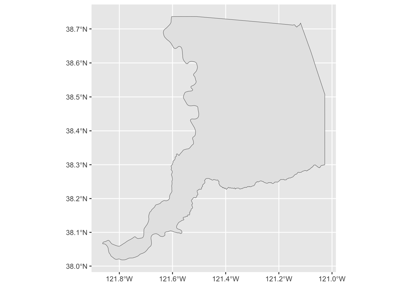
.dbf files are one kind of database file. If you’ve ever opened a shapefile with attribute information, you’ve used a .dbf file. The foreign package allows us to read .dbf files into R. Since this is a new package, we need to install it with install.packages("foreign").
We’ve been loading entire packages with the library() function, but you can also call a function from a package without loading it by using <package_name>::<function_name> syntax. Let’s load the .dbf file from our Sacramento County polygon.
foreign::read.dbf("data/shp/sac/sac_county.dbf").rds and .rda (.rda is shorthand for .RData) are a special R-based data formats used to store R objects. These files can be read just like another other import functions shown above. Let’s use it to import the groundwater level station data we read in earlier. Note that a .rds file can hold any single R object.
stations <- read_rds("data/gwl/stations.rds")
head(stations)
Sometimes, you may create an intermediate result that is time-consuming to recreate from scratch each time, and you want to save that intermediate result to streamline future analyses. You can export, or write this object to any number of data formats like a csv, SQL database, or shapefile. Unlike these data formats however, data saved as .rds are saved as one of R’s object classes, like data.frame, vector, list, and so on. In practice, only R is used to read .rds and .rda files, so these formats are chosen when we expect to use R to read these data at a later time.
One quick difference between .rds and .rda files, for .rds files we can only store a single R object (of any kind). For an .rda file, we can store many. .rda are also compressed by default. There are pros and cons we will discuss later.
SQLite is an open-source database format based on SQL that’s useful for storing large datasets locally on your computer. The methods to connect to a SQLite database, list tables, read tables, and send queries are similar across other cloud databases you may encounter in the wild, like Postgres, and enterprise database systems like Microsoft Access. We use the here package to construct relative paths in the RProject.
library(RSQLite)
library(here)
# location of an sqlite database
dbpath <- here("data/gwl/gwl_data.sqlite")

# actually connect to the database
dbcon <- dbConnect(dbDriver("SQLite"), dbpath)

# list all the tables in the database
dbListTables(dbcon)
[1] "measurements_sep" "perforations" "stations" # get one of the tables into a dataframe
head(dbReadTable(dbcon, "stations"))head(dbReadTable(dbcon, "measurements_sep"))# pass a query to the database
dbGetQuery(dbcon, "SELECT * from measurements_sep WHERE STN_ID = 4775 LIMIT 5")To write (export) data in R you need 2 things: data to write, and a location and format to write the data. For example, if we wanted to write our stations data to a csv in the “data_output” folder, we would do the following:
# write "stations" to a file in the data_output folder called "my_stations.csv"
write_csv(stations, "data_output/my_stations.csv")
Now check that location and verify that your station data was written.
We can do the same for other files:
# write the Sacramento county polygon to a shapefile
st_write(sac_county, "data_output/sac_county.shp")

# write the Sacramento county polygon to an rds file
write_rds(sac_county, "data_output/sac_county.rds")
As before, navigate to these folders to verify these data were written. We can also check to see if these data exist from within R:
my_results <- list.files("data_output")
my_files  <- c("sac_county.shp", "sac_county.rds")

# test if your files are in the data_output folder
my_files %in% my_results

# another handy function is `file.exists`, which tells you if your file exists
file.exists("data_output/sacramento_county.shp")
file.exists("data_output/sac_county.shp")
file.exists("data_output/sac_county.rds")
Challenge 2
breakfast and assign it a string with what you had for breakfast.breakfast.rds file in /data_output# create a string and write it to an rds file
breakfast <- "green eggs and ham"
# write_rds takes two arguments: the object to write and location to write it
write_rds(breakfast, "data_output/breakfast.rds")
# read the rds file back into R and save it as a variable
my_breakfast <- read_rds("data_output/breakfast.rds")
# use the `cat()` function (concatenate) to announce your breakfast
cat("Today for breakfast I ate", my_breakfast)