cms_to_cfs <- function(discharge) {
  cfs_out <- discharge * 35.3146662
  return(cfs_out)
}10 Function Junction
Functions
- Understand what a function is
- Understand how to use functions in R
- Write your own simple function
10.1 Functions
What is a function? A function is simply a set of instructions or code written for a computer to follow. These can be very simple (multiply one column of data by another) to much more complex (multi-step model and visualization). Packages are usually sets of functions that focus on similar topics or themes, sort of like a cookbook for a specific kind of food.
Functions ultimately make our code more reusable and reproducible, because we can use functions for repeated processes (like cleaning and tidying data!).
10.1.1 What’s in a Function?
In R, functions have a name, an input which may consist of one or more arguments (sometimes called parameters) and a output or the thing that the function returns.
Here’s an example function to convert discharge from cubic meters per second (cms) to cubic feet per second (cfs). Can you identify the different parts?
10.1.2 Running a Function
Using functions requires we know what pieces go where inside the function (the arguments), our data is of the right class or shape for the function (input), and we know what the function should return to our Environment! Once we have this basic understanding, there are thousands of functions that are already written and part of packages we can use. In fact, we’ve been using functions in every lesson thus far. In this module, we focus on building our own functions to meet our data science needs.
To use the cms_to_cfs function we wrote above, we need to provide a value to the discharge argument. Let’s convert 10 cms to cfs, using our function.
cms_to_cfs(discharge = 10)[1] 353.1467The function returns a numeric value to our console. If we wanted to save this value, we could assign it (<-) to an object. Functions allow us to iterate over data, or repeat the same task on different datasets without needing to re-write code every time.
10.1.3 Naming Functions in R
It’s important to adopt consistent and descriptive names in R. This isn’t just for functions, but it’s a particularly good habit to practice when naming functions. For example, a general recommendation is to 🐍 use_snake_case 🐍. Other options include:
MaybeUseCamelCaseor.separate.by.periodsorJust_try.everythingBecause.CHAOS
10.2 Use a Function from a Package
We’ve already been doing this throughout the previous lessons with things like read.csv(), dplyr::filter(), or ggplot2::ggplot(), but let’s use a new package to pull some surface water river flow data. Here we’ll use the dataRetrieval package.
10.2.1 Getting Water Data with dataRetrieval
The {dataRetrieval} package is a way to access hydrologic and water quality data from the USGS and EPA. There are several vignettes (or tutorials) available on the package website. Here, we will show how to download some surface water data from the American River near Sacramento. First we load the package with the functions we want to use. We load packages once per session.
# load the functions via packages!
library(tidyverse)
library(dataRetrieval) # a spellbook of water data functions

# use a function to download data:
flow_site <- readNWISdata(site = "11427000", # USGS Station ID
                          service = "iv", # instantaneous measurements
                          parameterCd = "00060", # discharge in cfs
                          startDate = "2019-10-01",
                          endDate = "2021-09-30",
                          tz = "America/Los_Angeles")
There are a lot of arguments in that function! How did we know what each one was or what to put there? There are a few different options. For functions or packages you aren’t familiar with, it’s worth using built-in help.
- Look up help for a function with
?readNWISdataand look at theUsageandArgumentssections! - Use tab autocomplete as much as you can in RStudio! Once inside a function’s parenthesis, hit tab! There are generally a list of arguments that will pop up, each with some info about them. This is the same info we should find in the Help tab when we look up the function.
10.2.2 How do we know it worked?
Always visualize and inspect your data… we should have an object in our environment called flow_site. Let’s take a look at this data, tidy it, and plot!
# check data
summary(flow_site)
agency_cd site_no dateTime
Length:70080 Length:70080 Min. :2019-10-01 00:00:00
Class :character Class :character 1st Qu.:2020-03-31 13:26:15
Mode :character Mode :character Median :2020-09-30 13:07:30
Mean :2020-09-30 12:39:55
3rd Qu.:2021-04-01 11:48:45
Max. :2021-09-30 23:45:00
X_00060_00000 X_00060_00000_cd tz_cd
Min. : 9.68 Length:70080 Length:70080
1st Qu.: 55.50 Class :character Class :character
Median : 115.00 Mode :character Mode :character
Mean : 323.72
3rd Qu.: 411.00
Max. :4580.00 head(flow_site)# fix column names so we can use a more informative parameter name
flow_site <- dataRetrieval::renameNWISColumns(flow_site)
# check data
names(flow_site)[1] "agency_cd" "site_no" "dateTime" "Flow_Inst" "Flow_Inst_cd"
[6] "tz_cd" # visualize:
ggplot(data = flow_site) +
geom_line(aes(x = dateTime, y = Flow_Inst), color = "darkblue") +
theme_classic() +
labs(x = "", y = "Flow (cfs)",
title = "Discharge from USGS Station 11427000",
caption = "data pulled using {dataRetrieval} package in R")
Awesome! We plotted some discharge data from a river. That’s great. We could save this data if we wanted (see the import/export module), or do additional analysis (see next module on joins!). Let’s try using a different function here.
Challenge 1: You Try!
Using the code template below, create a
flow_hucobject using thereadNWISdata()function but fill in the arguments with the following information:- Instead of
site, let’s usehuc. We’ll try getting stations from HUC 18020111. - Instead of
iv(instantaneous), let’s usedv. - Use the same
startDate,endDate, andparameterCdas we used above. %>%the output fromreadNWISdata()directly to therenameNWISColumns()function and then to theaddWaterYear()function.
- Instead of
How many unique
site_noare there?Can you visualize the data using a
ggplot()withgeom_lineand use a different color for eachsite_no?
Code template:
flow_huc <- readNWISdata(___,
                         ___,
                         parameterCd = "00060",
                         startDate = "2019-10-01",
                         endDate = "2021-09-30") %>%
  ___ %>%
  ___
Click for Answers!
# look for stations with daily values of discharge in the whole watershed
flow_huc <- readNWISdata(huc = "18020111", # using a huc id number now
                         service = "dv", # daily values
                         parameterCd = "00060",
                         startDate = "2019-10-01",
                         endDate = "2021-09-30") %>%
  renameNWISColumns() %>%  # the pipe infers that the data is passed through
  addWaterYear()

names(flow_huc) # names look ok!
[1] "agency_cd" "site_no" "dateTime" "waterYear" "Flow" "Flow_cd"
[7] "tz_cd" unique(flow_huc$site_no) # 2 stations[1] "11446500" "11447360"# visualize:
ggplot() +
geom_line(data = flow_huc,
aes(x = dateTime, y = Flow, color = site_no),
show.legend = FALSE) +
theme_classic() +
labs(x = "", y = "Flow (cfs)",
title = "Discharge from USGS Stations: 11446500, 11447360",
caption = "data pulled using {dataRetrieval} package in R") +
# a new way to view data with facets...add a free scale!
facet_grid(rows = vars(site_no), scales = "free") 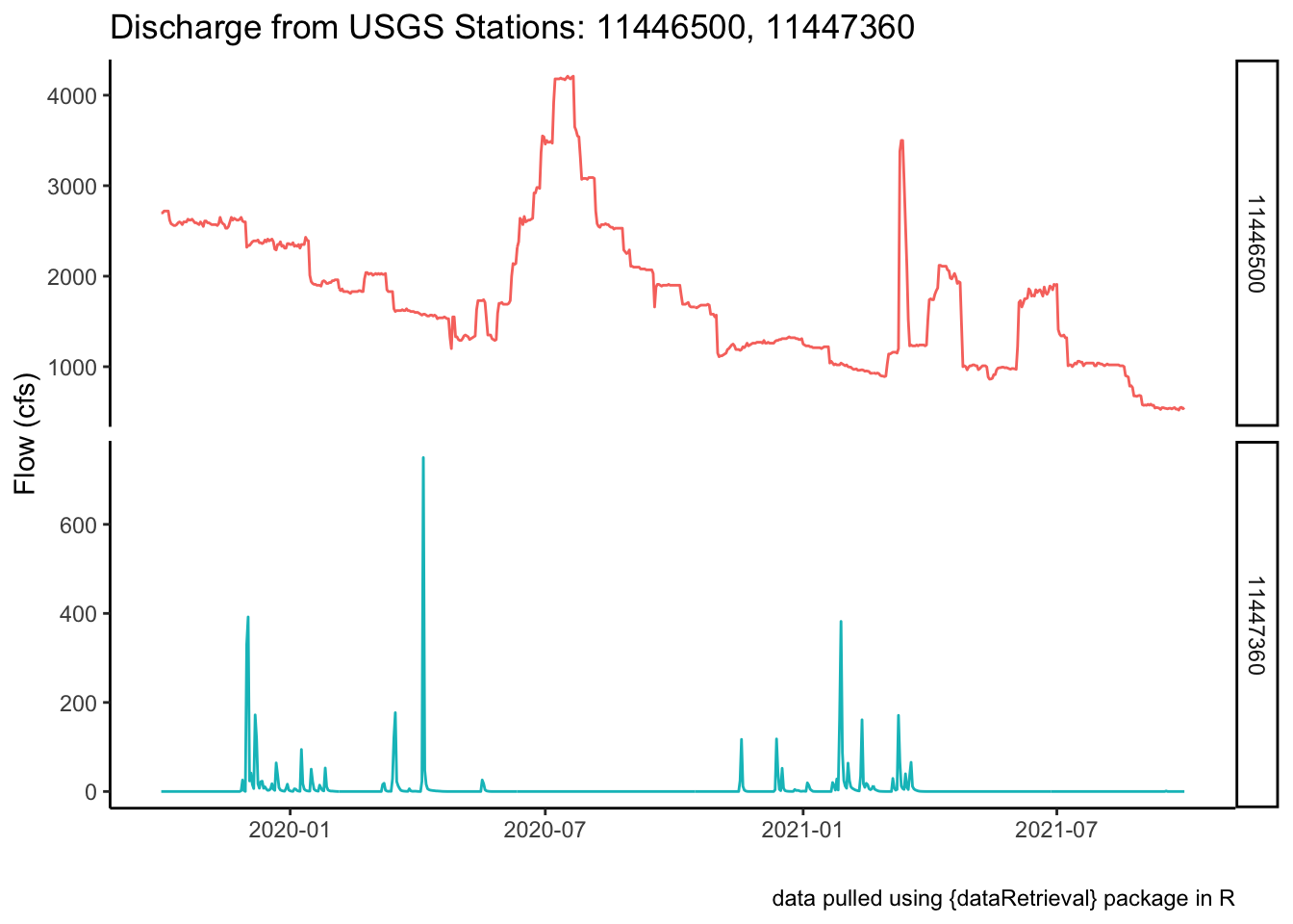
10.3 Using Custom Functions
Since we already wrote a custom function to convert cms to cfs, let’s make another similar function but for cfs to cms, and apply it to the flow data we just downloaded. Let’s look at how we might use a function on an existing data frame or dataset that we have in R.
10.3.1 Convert Flow Data to cms
Let’s use some of the dplyr we looked at in the last lesson. Here we want to make a new column that is our Flow data, but instead of in cfs, our units will be in cms. Let’s use the flow_site data frame.
# the function
cfs_to_cms <- function(discharge) {
  cms_out <- discharge * 0.028316847
  return(cms_out)
}

# add a new column to existing dataset with mutate
flow_site <- flow_site %>%
  mutate(Flow_cms = cfs_to_cms(Flow_Inst)) # apply the function to the column

# quick plot to check!
ggplot() +
  geom_line(data = flow_site,
            aes(x = dateTime, y = Flow_cms), color = "darkblue") +
  theme_classic() +
  labs(x = "", y = "Flow (cms)",
       title = "Discharge from USGS Station 11427000",
       caption = "data pulled using {dataRetrieval} package in R")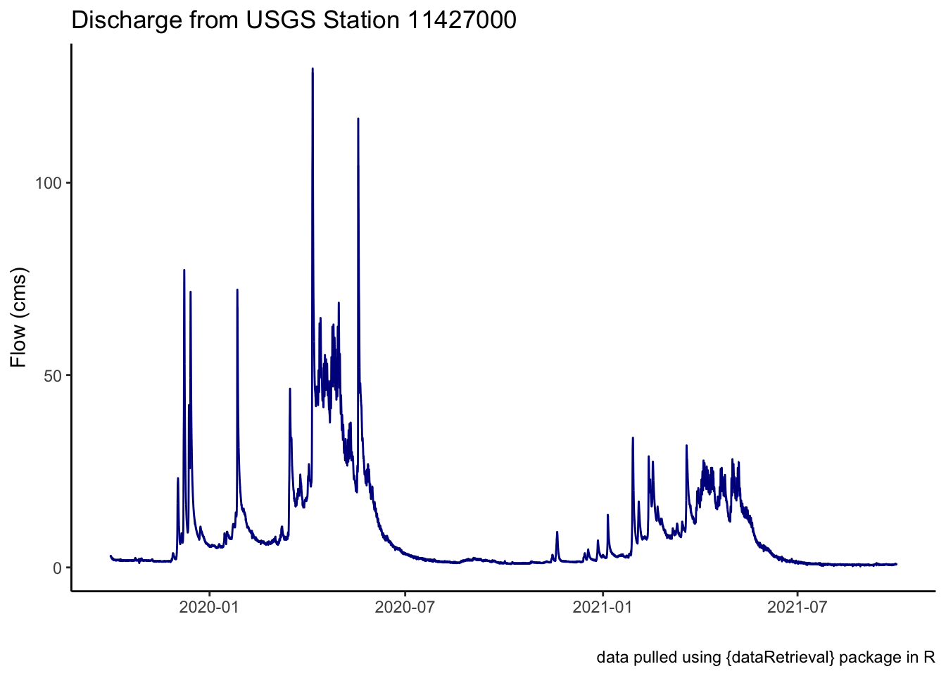
So what happened here? We made a function cfs_to_cms() to apply to our data. In this case, we wanted to apply our function to a column in our dataframe, which if we remember the earlier lesson on data, in a dataframe a column is a vector of the same type of data. That means the function can very quickly iterate through every observation in the vector and convert the data from cfs to cms.
10.4 More Practice
This section uses some more functions, but with some more advanced applications. We’ll want to have the sf package installed for the following code to work fully.
10.4.1 Getting Water Quality Stations
What if we wanted to find all the possible water quality stations that are upstream or downstream of the gage we pulled data from earlier (USGS: 11446500)? A great function that will not only help us figure that out, but also help us pull in spatial data we can use to make maps is the findNLDI() function from the dataRetrieval package.
The function findNLDI() has arguments for the type of data we want to use (nwis, huc,location), the direction along a stream to look (upstream or downstream, or in mainstem or tributaries), the data we want to get back (find), and the distance we should search upstream or downstream (distance_km).
Let’s look only in the mainstem river for 50 km upstream or downstream of our USGS gage and return any NWIS (water quality or flow) sites and the associated flowlines we searched.
library(sf)

# get NWIS and flowline data 50km downstream of the USGS gage
amer_ds_nimbus <- findNLDI(
  nwis = "11446500", # Below Nimbus Dam
  nav = c("UM","DM"),
  find = c("nwis", "flowlines"),
  distance_km = 50)

names(amer_ds_nimbus)
[1] "origin" "UM_nwissite" "UM_flowlines" "DM_nwissite" "DM_flowlines"Note, this returned a named list of dataframes. We can access individual parts of a list just as we can access a single column in a dataframe using the $. This function returned 5 parts, the origin which is the site we used to start our search, the UM_nwissite which is the NWIS sites upstream on the mainstem from our USGS gage, the DM_nwissite which is the NWIS sites downstream of our USGS gage, and finally, a mainstem flowline upstream and downstream of our gage. These are dataframes with an underlying spatial component, which is nice because it allows us to easily map and visualize these data if we want. See the mapmaking lesson for more info.The dataframes are an sf class, from the simple features sf package, but they can also be converted to into a dataframe.
# check the object class
class(amer_ds_nimbus$DM_nwissite)
[1] "sf" "tbl_df" "tbl" "data.frame"# get just downstream NWIS sites and make into dataframe
nwis_sites <- amer_ds_nimbus$DM_nwissite %>%
st_drop_geometry() # drop the sf class
# verify the class has changed
class(nwis_sites)[1] "tbl_df" "tbl" "data.frame"Let’s visualize these sites with a fancy map! See the mapmaking lesson for more details on making maps in R.
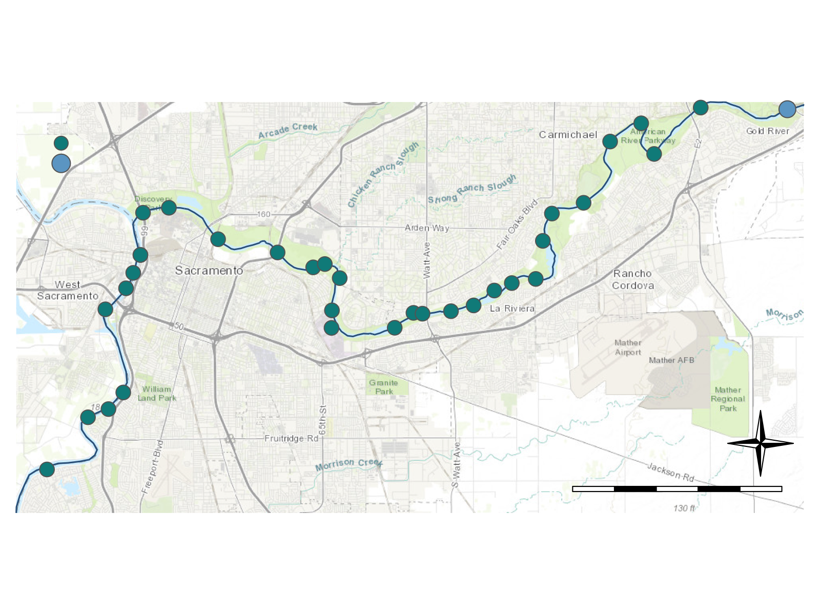
10.4.2 Save Our Data!
Finally, let’s go ahead and save (export) our list of NWIS sites, and all our spatial components from the American River below Nimbus Dam so we can use it for future lessons.
# save out
write_csv(nwis_sites, path = "data/nwis_sites_american_river.csv")
write_rds(amer_ds_nimbus, path = "data/nwis_sites_amer_ds_nimbus_sf.rds")
10.5 Additional Water Packages of Interest
There are many packages that work with water or water data. Here’s a list of just a few that you may find interesting or helpful. The R CRAN repository has a list of all packages that relate to Hydrology that is also a good place to look.
dataRetrievalnhdplusToolsEGRETgeoknife