# GENERAL PACKAGES
library(tidyverse) # data wrangling & viz
library(purrr) # iteration
library(janitor) # name cleaning
library(glue) # pasting stuff together

# SPATIAL PACKAGES
library(sf) # analysis tools
library(mapview)  # interactive maps!
mapviewOptions(fgb = FALSE) # to save interactive maps

library(tigris) # county & state boundaries
library(units) # for convert spatial and other units
library(dataRetrieval) # download USGS river data
library(tmap) # mapping
library(tmaptools) # mapping tools23 Advanced spatial R and mapmaking: I
Learning objectives
- Learn to extend and use
sffor geospatial work - Understand the power of script-based geospatial/mapping
- Expand your geospatial skills in R!
23.1 Overview
The ability to work in one place or with one program from start to finish is powerful and more efficient than splitting your workflow across multiple tools. By sticking with one single framework or set of tools, we can reduce the mental workload necessary when switch between programs, staying organized in each, and dealing with import/export across multiple programs. Although different tools such as ESRI (or ArcPy extensions) are powerful, they require a paid license and typically use point-click user interfaces.
The advantage R has over these tools is that it is freely available, easily integrates with vast statistical/modeling toolboxes, has access to many spatial analysis and mapmaking tools, and allows us to work in a single place.
If we use a functional programming approach (described in the iteration module ) for spatial problems, R can be a very robust and powerful tool for analysis and spatial visualization of data! Furthermore, once analyses have been completed, we can re-use the scripts and functions for common spatial tasks (like making maps or exporting specific spatial files).
23.1.1 Common Geospatial Tasks
Common tasks in a GUI-based approach will always require the same number of point and clicks. With a script-based approach, it’s much easier to recycle previously written code, or to just change a variable and re-run the code. This efficiency is magnified immensely when it can be automated or iterated over the same task through time, or multiple data sets.
For example, some common tasks may include:
- Cropping data to an area of interest for different users
- Reproducing a map with updated data
- Integrating or spatial joining of datasets
- Reprojecting spatial data
23.1.1.1 Script-based analyses with sf
The sf package truly makes working with vector-based spatial data easy. We can use a pipeline that includes:
st_read(): read spatial data in (e.g., shapefiles)st_transform(): transform or reproject datast_buffer(): buffer around datast_union(): combine data into one layerst_intersection(): crop or intersect one data by anothergroup_split()&st_write()to split data by a column or attribute and write out
There are many more options that can be added or subtracted from these pieces, but at the core, we can use this very functional approach to provide data, make maps, conduct analysis, and so much more.
23.2 A Groundwater/Surfacewater Hydrology Example
Let’s use an example where we read in some groundwater station data, spatially find the closest surface water stations, download some river data, and visualize!
23.2.1 The Packages
First we’ll need a few packages we’ve not used yet. Please install these with install.packages() if you don’t have them.
23.2.2 Importing Spatial Data
We’ll leverage the ability to pull in many different data and stitch them all together through joins (spatial or common attributes). Each data component may be comprised of one or more “layers”, which ultimately we can use on a map.
23.2.2.1 Get State & County Data
First we need state and county boundaries. The tigris package is excellent for this.
# get {sf} CA boundary
ca <- states(cb=TRUE, progress_bar = FALSE) %>%
  dplyr::filter(STUSPS == "CA")

# get counties for CA as {sf}
ca_co <- counties("CA", cb = TRUE, progress_bar = FALSE)
Let’s also pull in a shapefile that’s just Sacramento County. We’ll use this to crop/trim things down as we move forward. Note, we’ll need to check the coordinate reference system and projection here, and make sure we are matching our spatial data.
# get just sacramento: here we read in a shapefile:
sac_co <- st_read("data/shp/sac/sac_county.shp")
Reading layer `sac_county' from data source
`/Users/richpauloo/Documents/GitHub/r4wrds/quarto-book/intermediate/data/shp/sac/sac_county.shp'
using driver `ESRI Shapefile'
Simple feature collection with 1 feature and 9 fields
Geometry type: POLYGON
Dimension: XY
Bounding box: xmin: -13565710 ymin: 4582007 xmax: -13472670 ymax: 4683976
Projected CRS: WGS 84 / Pseudo-Mercator# check CRS
st_crs(sac_co)$epsg[1] 3857# match with other data
sac_co <- st_transform(sac_co, st_crs(ca_co))
st_crs(sac_co) == st_crs(ca_co) # should be TRUE![1] TRUE# make a box around sacramento county
# (a grid with an n=1) for inset
sac_box <- st_make_grid(sac_co, n = 1)And let’s quickly visualize these pieces! We’ll use the base plot() functions here.
# make sure we have all the pieces with a quick test plot
plot(ca$geometry, col = alpha("gray", 0.5), border = "black", lwd=2)
plot(ca_co$geometry, add = T, border = "purple", col = NA)
plot(sac_co$geometry, add = T, border = "cyan4", col = "skyblue",alpha=0.4, lwd = 2)
plot(sac_box, add = T, border = "orange", col = NA, lwd = 1.4)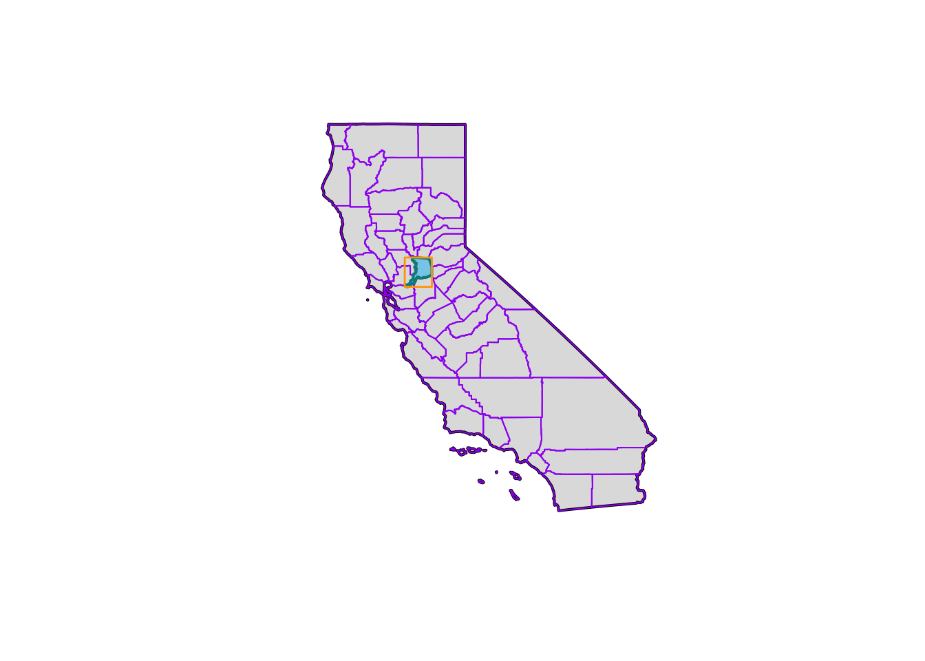
23.2.2.2 Iterate: Get Groundwater Stations
Let’s practice our iteration skills. We’ll read in groundwater stations for 3 counties (El Dorado, Placer, and Sacramento), convert to sf objects, plot them, and then crop/select a subset of stations using spatial intersection.
Iteration…remember purrr? Let’s use it here!
# read the stations
gw_files <- list.files(path = "data/gwl/county",
                       full.names = TRUE, pattern = "*.csv")

# read all files into dataframes and combine with purrr
gw_df <- map_df(gw_files, ~read.csv(.x))

# the readr package will also do this same thing by default
# when passed a list of files with the same data types
gw_df <- read_csv(gw_files)

# now make "spatial" as sf objects
gw_df <- st_as_sf(gw_df, coords=c("LONGITUDE","LATITUDE"),
                  crs=4326, remove=FALSE) %>%
  # and transform!
  st_transform(., st_crs(ca_co))

# preview!
mapview(gw_df, zcol="COUNTY_NAME", layer.name="GW Stations") +
  mapview(sac_co, legend=FALSE)
Hmmm…looks like there are some stations up near Lake Tahoe, and then all the stations that are outside of the Sacramento County boundary. Let’s move on to do some cleaning/cropping/joining.
23.2.3 Filter, Select, & Spatial Joins
One of the more common spatial operations is filtering or clipping data based on a condition or another spatial layer.
Often to complete a geospatial operation, we need to use a projected coordinate reference system1 (not latitude/longitude), so we can specify things in units that are easier to understand (kilometers or miles) instead of arc degrees, and so that the calculations take place correctly. Note, here we have transformed our data to match up.
23.2.3.1 Filter
We could certainly leverage the data.frame aspect of sf and quickly filter down to the stations of interest using the COUNTY_NAME field.
You Try!
Use filter() to filter our gw_df dataframe to only stations that occur in Sacramento County. Then make a mapview() map and make the color of the dots correspond with the different WELL_USE categories. How many stations are there in each WELL_USE category?
Click for Answers!
gw_sac <- gw_df %>%
  filter(COUNTY_NAME == "Sacramento")

table(gw_sac$WELL_USE)
   Industrial    Irrigation   Observation         Other   Residential
            2           144            90           101            76
Stockwatering       Unknown
6 67 mapview(gw_sac, zcol="WELL_USE", layer.name="Well Use")23.2.3.2 Spatial Crop
Great! But what if we don’t have the exact column we want, or any column at all? We may only have spatial data, and we want to trim/crop by other spatial data. Time for spatial operations.
First, we can use base [] to crop our data. Here we take the dataset we want to crop or clip (gw_sac) and crop by the Sacramento county polygon (sac_co). This is a type of spatial join, but note, we retain the same number of columns in the data.
# spatial crop:
# # does not bring attributes from polygons forward
gw_sac_join1 <- gw_df[sac_co,]

plot(sac_co$geometry, col = alpha("forestgreen", 0.6))
plot(gw_sac_join1$geometry, bg = alpha("orange", 0.3), pch=21, add = TRUE)
title("GW Stations (orange) \nthat occur in Sacramento County")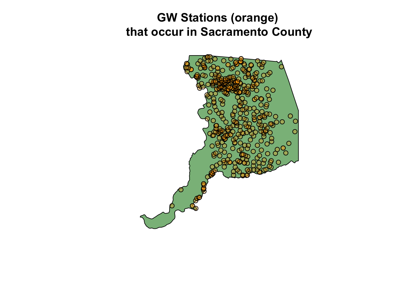
23.2.3.3 Spatial Join
We can also use st_join() directly to filter for points that fall within a supplied polygon(s). In our case, we want groundwater stations (points) that fall within our selected counties (polygons).
gw_sac_join2 <- st_join(gw_df, sac_co, left = FALSE)

mapview(gw_sac_join2, col.region="orange", legend=FALSE) +
  mapview(sac_co, alpha = 0.5, legend = FALSE)
Note, what’s different between gw_df and gw_sac_join1?
We can also use an anti_join (the !) to find the stations that weren’t contained in our focal area. These operations can be helpful when exploring and understanding a dataset, to identify gaps, highlight specific areas, etc. st_intersects returns a vector of items based on whether the two spatial objects intersect (which can be defined differently using a multitude of spatial functions, see the sf help page).
# anti_join: find stations that aren't contained in Sacramento County
gw_sac_anti <- gw_df[!lengths(st_intersects(gw_df, sac_co)), ]

# plot
mapview(gw_sac_anti,
        col.regions="maroon", cex=3,
        layer.name="Anti-Join Sites") +
  mapview(sac_co, alpha.regions=0,
          color="black", lwd=3, legend=FALSE)
23.2.4 Writing Spatial Data Out
We may want to save these data and send to colleagues before we proceed with further analysis. As we’ve shown before2, functional programming allows us to split data and write it out for future use, or to share and distribute. Here we use a fairly simple example, but the concept can be expanded.
Let’s use the purrr package to iterate over a lists and write each layer to a geopackage (a self contained spatial database). Geopackages are a great way to save vector-based spatial data, they can be read by ArcGIS and spatial software, and they are compact and self-contained (unlike shapefiles).
library(purrr)
library(glue)
library(janitor)

dir.create("data_output", showWarnings = FALSE, recursive = TRUE)

# first split our gw_df data by county:
gw_df_split <- gw_df %>%
  split(.$COUNTY_NAME) %>% # split by cnty name
  set_names(., make_clean_names(names(.))) # make a file friendly name

# now apply function to write out points by county
map2(gw_df_split, # list of points by county
     names(gw_df_split), # list of names for layers
     ~st_write(.x,
               dsn = "data_output/county_gw_pts.gpkg",
               layer = glue("{.y}_gw_pts"),
               delete_layer=TRUE, # to remove layer if it exists
               quiet = TRUE) # suppress messages
     )
$el_dorado
Simple feature collection with 45 features and 14 fields
Geometry type: POINT
Dimension: XY
Bounding box: xmin: -120.07 ymin: 38.80169 xmax: -119.944 ymax: 38.95919
Geodetic CRS: NAD83
# A tibble: 45 × 15
STN_ID SITE_CODE SWN WELL_NAME LATITUDE LONGITUDE WLM_METHOD WLM_ACC
<dbl> <chr> <chr> <chr> <dbl> <dbl> <chr> <chr>
1 10713 388017N1200185W… 11N1… <NA> 38.8 -120. Unknown Unknown
2 47508 388030N1200150W… <NA> EX-1 38.8 -120. Surveyed … 0.1 ft.
3 47519 388224N1200217W… 11N1… SUT No.1 38.8 -120. Surveyed … 0.1 ft.
4 47510 388395N1200249W… <NA> Henderso… 38.8 -120. Surveyed … 0.1 ft.
5 47504 388544N1200196W… <NA> DW-1 38.9 -120. Surveyed … 0.1 ft.
6 47512 388545N1200196W… <NA> IW-1 38.9 -120. Surveyed … 0.1 ft.
7 47520 388545N1200197W… <NA> SW-1 38.9 -120. Surveyed … 0.1 ft.
8 47499 388552N1200171W… <NA> Apache OW 38.9 -120. Surveyed … 0.1 ft.
9 15199 388562N1200143W… 12N1… <NA> 38.9 -120. Unknown Unknown
10 47506 388582N1200216W… <NA> ESB-2 38.9 -120. Surveyed … 0.1 ft.
# ℹ 35 more rows
# ℹ 7 more variables: BASIN_CODE <chr>, BASIN_NAME <chr>, COUNTY_NAME <chr>,
# WELL_DEPTH <dbl>, WELL_USE <chr>, WELL_TYPE <chr>, geometry <POINT [°]>
$placer
Simple feature collection with 184 features and 14 fields
Geometry type: POINT
Dimension: XY
Bounding box: xmin: -121.614 ymin: 38.7005 xmax: -120.112 ymax: 39.3079
Geodetic CRS: NAD83
# A tibble: 184 × 15
STN_ID SITE_CODE SWN WELL_NAME LATITUDE LONGITUDE WLM_METHOD WLM_ACC
<dbl> <chr> <chr> <chr> <dbl> <dbl> <chr> <chr>
1 48577 381626N1213651W… <NA> SVMW Eas… 38.8 -121. Surveyed … 0.1 ft.
2 55217 387005N1216141W… <NA> Elkhorn … 38.7 -122. Unknown Unknown
3 55218 387005N1216141W… <NA> Elkhorn … 38.7 -122. Unknown Unknown
4 33091 387216N1212470W… 10N0… 10N07E18… 38.7 -121. Unknown Unknown
5 52475 387222N1212920W… <NA> Whyte A 38.7 -121. GPS 0.1 ft.
6 52476 387222N1212920W… <NA> Whyte B 38.7 -121. GPS 0.1 ft.
7 13664 387269N1212760W… 10N0… <NA> 38.7 -121. Unknown Unknown
8 13665 387285N1213396W… 10N0… <NA> 38.7 -121. Unknown Unknown
9 13670 387290N1212518W… 10N0… <NA> 38.7 -121. Unknown Unknown
10 51280 387331N1213610W… <NA> WPMW-5A 38.7 -121. Surveyed … 0.1 ft.
# ℹ 174 more rows
# ℹ 7 more variables: BASIN_CODE <chr>, BASIN_NAME <chr>, COUNTY_NAME <chr>,
# WELL_DEPTH <dbl>, WELL_USE <chr>, WELL_TYPE <chr>, geometry <POINT [°]>
$sacramento
Simple feature collection with 494 features and 14 fields
Geometry type: POINT
Dimension: XY
Bounding box: xmin: -121.695 ymin: 38.1023 xmax: -121.043 ymax: 38.7311
Geodetic CRS: NAD83
# A tibble: 494 × 15
STN_ID SITE_CODE SWN WELL_NAME LATITUDE LONGITUDE WLM_METHOD WLM_ACC
<dbl> <chr> <chr> <chr> <dbl> <dbl> <chr> <chr>
1 49420 380926N1215871W… 03N0… 03N03E12… 38.1 -122. GPS 10 ft.
2 49421 380926N1215871W… 03N0… 03N03E12… 38.1 -122. GPS 10 ft.
3 49419 381023N1215691W… 03N0… 03N03E12… 38.1 -122. GPS 10 ft.
4 49425 381123N1215102W… 03N0… 03N04E16… 38.1 -122. GPS 10 ft.
5 49426 381123N1215102W… 03N0… 03N04E16… 38.1 -122. GPS 10 ft.
6 50577 381132N1216951W… 03N0… COSAC3 38.1 -122. Digital E… 0.1 ft.
7 49423 381170N1215245W… 03N0… 03N04E17… 38.1 -122. GPS 10 ft.
8 49433 381200N1214920W… 03N0… 03N04E13… 38.1 -121. GPS 10 ft.
9 49428 381222N1214999W… 03N0… 03N04E11… 38.1 -122. GPS 10 ft.
10 49416 381301N1215640W… 03N0… 03N04E02… 38.1 -122. GPS 10 ft.
# ℹ 484 more rows
# ℹ 7 more variables: BASIN_CODE <chr>, BASIN_NAME <chr>, COUNTY_NAME <chr>,
# WELL_DEPTH <dbl>, WELL_USE <chr>, WELL_TYPE <chr>, geometry <POINT [°]>To make sure this worked as intended, we can check what layers exist in the geopackage with the st_layers function.
# check layers in the gpkg file
st_layers("data_output/county_gw_pts.gpkg")
23.3 Additional Resources
We’ve covered a handful of packages and functions in this module, but many more exist that solve just about every spatial workflow task. All spatial and mapmaking operations are typically a websearch away, but we also recommend the following resources to dig deeper into the R spatial universe.
A discussion on coordinate reference systems is a complex topic in and of itself, and for the purposes of this module, we summarize it as follows: A geographic CRS is round and based on angular units of degrees (lat/lng), whereas a projected CRS is flat and has linear units (meters or feet). Many functions in
sfthat make calculations on data expect a projected CRS, and can return inaccurate results if an object in a geographic CRS is used. This is a fascinating topic with lots written about it! For more reading see this Esri blog, the Data Carpentry geospatial lesson, and the online Geocomputation with R book.↩︎See the iteration module for an example of iterating over a write function.↩︎