# GENERAL PACKAGES
library(tidyverse) # data wrangling & viz
library(purrr) # iteration
library(janitor) # name cleaning
library(glue) # pasting stuff together

# SPATIAL PACKAGES
library(sf) # analysis tools
library(mapview)  # interactive maps!
mapviewOptions(fgb = FALSE) # to save interactive maps

library(tigris) # county & state boundaries
library(units) # for convert spatial and other units
library(dataRetrieval) # download USGS river data
library(tmap) # mapping
library(tmaptools) # mapping tools24 Advanced spatial R and mapmaking: II
Learning objectives
- Learn to extend and use
sfwith aquatic data from NHD sources - Mapping with
tmap - Advanced spatial operations with vector data
24.1 Overview
We can use some of the same tools and data we used previously, but we can now also add a few options to download and actively use USGS/NHD data. These data include river stage and flow, water quality, station locations, watershed and streamline attributes, etc. Particularly for water scientists, it can be immensely useful to tie in additional data, or use standard datasets that are continuously updated (like the USGS gage network).
24.1.1 The Packages
First we’ll need a few packages we’ve not used yet. Please install these with install.packages() if you don’t have them.
24.1.2 River Data: Find Nearest USGS Station
We’ve demonstrated how to join data and crop data in R, but let’s use some alternate options to download new data. We’ll focus on surface water here, and look at how we can download and map flowlines in R. Much of the USGS data network can be queried and downloaded in R. This may include data on water quality, river discharge, water temperature, spatial basins, and NHD flowlines. The dataRetrieval package is an excellent option for these operations.
Let’s find a few groundwater stations to use. Here we’ll grab one close to the American River and one close to the Cosumnes just for demonstration purposes, but this could be any X/Y point, or set of points you are interested in.
24.1.2.1 Groundwater Data
Iteration…remember purrr? Let’s use it here!
# get counties for CA as {sf}
ca_co <- counties("CA", cb = TRUE, progress_bar = FALSE)


# read the stations
gw_files <- list.files(path = "data/gwl/county",
                       full.names = TRUE, pattern = "*.csv")

# read all files into dataframes and combine with purrr
gw_df <- map_df(gw_files, ~read.csv(.x))

# the readr package will also do this same thing by default
# when passed a list of files with the same data types
gw_df <- read_csv(gw_files)

# now make "spatial" as sf objects
gw_df <- st_as_sf(gw_df, coords=c("LONGITUDE","LATITUDE"),
                  crs=4326, remove=FALSE) %>%
  # and transform!
  st_transform(., 4269)
Get the Sacramento County shapefile.
# get just sacramento: here we read in a shapefile:
sac_co <- st_read("data/shp/sac/sac_county.shp")
Reading layer `sac_county' from data source
`/Users/richpauloo/Documents/GitHub/r4wrds/quarto-book/intermediate/data/shp/sac/sac_county.shp'
using driver `ESRI Shapefile'
Simple feature collection with 1 feature and 9 fields
Geometry type: POLYGON
Dimension: XY
Bounding box: xmin: -13565710 ymin: 4582007 xmax: -13472670 ymax: 4683976
Projected CRS: WGS 84 / Pseudo-Mercator# check CRS
st_crs(sac_co)$epsg[1] 3857# match with other data
sac_co <- st_transform(sac_co, st_crs(ca_co))
st_crs(sac_co) == st_crs(ca_co) # should be TRUE![1] TRUE# make a box around sacramento county
# (a grid with an n=1) for inset
sac_box <- st_make_grid(sac_co, n = 1)Now we can filter to our location of interest.
# filter to only Sacramento
gw_sac <- gw_df %>%
  filter(COUNTY_NAME == "Sacramento")

# use this layer to filter to only locations (stations of interest)
sac_loi <- gw_sac %>% filter(STN_ID %in% c("52418", "5605"))

mapview(sac_co, alpha.regions=0,
          color="black", lwd=3, legend=FALSE) +
  mapview(sac_loi, col.regions="purple",layer.name="Locations of Interest")
24.1.2.2 Use findNLDI
The findNLDI function allows us to pass a single spatial point as well as a few different parameters like search upstream or downstream, and what we want to find, and then return a list of items (see the help page for using the function here), leveraging the hydro-network linked data index (NLDI)1. Note, we’ll need internet connectivity here for these functions to run successfully.
Let’s look only at mainstem flowlines from our locations of interest, and return the nearest NWIS sites as well as the NHD flowlines (streamlines). We’ll use the map() function to pass a list of stations along (here only 2, but this is flexible, and in practice we can map over a much larger number of stations).
First, we want to look up the COMID or location identifier for the centroids.
library(dataRetrieval)

# Need to convert our locations of interest to WGS84
sac_loi <- sac_loi %>%
  st_transform(4326)

# now we can go get flowline data!
us_nwis <- map(sac_loi$geometry,
                ~findNLDI(location = .x,
                          nav  = c("UM"),
                          find = c("nwis", "flowlines"),
                          distance_km = 120)
                )
Great, now we have a list of three or more things for each sf object we passed to findNLDI. In this case, we should have (for each location of interest we used):
origin: this is the segment that the original LOI was linked to based on the nearest distance algorithm the function used. Note, this is ansf LINESTRINGdata.frame.UM_nwissite: these are all the NWIS sites that were identified upstream of our origin point.UM_flowlines: these are the Upstream Mainstem (UM) flowlines from our origin point.
Let’s play with these data and make some maps.
24.1.2.3 Extract the NLDI Info
There are a few options, and it depends on what your goal is. Here we show a few simple ways to pull these data out or collapse them. Remember, we can access things in lists with our [[]] too!
# we can split these data into separate data frame
# and add them as objects to the .Global environment.
# first add names based on our station IDs:
us_nwis <- set_names(us_nwis, nm=glue("id_{sac_loi$STN_ID}"))

# then split into separate dataframes
# us_nwis %>% list2env(.GlobalEnv)

# Or we can combine with map_df
us_flowlines <- map_df(us_nwis, ~rbind(.x$UM_flowlines))
us_nwissite <- map_df(us_nwis, ~rbind(.x$UM_nwissite))

mapview(sac_loi, col.region="purple", legend = TRUE,
        cex=3, layer.name="GW LOI") +
  mapview(us_nwissite, col.regions="orange",
          legend = TRUE, layer.name="UM NWIS Sites") +
  mapview(us_flowlines, color="steelblue", lwd=2,
          layer.name="UM Flowlines", legend=FALSE)
Next, let’s filter to NWIS USGS stations that have flow data (generally these have 8-digit identifiers instead of a longer code which can be more water quality parameters), and pull streamflow data for the nearest station.
# use the stringr package, part of tidyverse to trim characters
usgs_stations <- us_nwissite %>%
  filter(stringr::str_count(identifier) < 14)

# double check?
mapview(sac_loi, col.region="purple", legend = TRUE,
        cex=3, layer.name="GW LOI") +
  mapview(us_nwissite, col.regions="orange", cex=2,
          legend = TRUE, layer.name="UM NWIS Sites") +
  mapview(usgs_stations, col.regions="cyan4",
          legend = TRUE, layer.name="USGS Gages") +
  mapview(us_flowlines, color="steelblue", lwd=2,
          layer.name="UM Flowlines", legend=FALSE)
24.1.2.4 Snap to the Nearest Point
The final filter involves snapping our LOI points (n = 2) to the nearest USGS stations from the stations we filtered to above. We can then use these data to generate some analysis and exploratory plots.
Snapping spatial data can be tricky, mainly because decimal precision can cause problems. One solution is to add a slight buffer around points or lines to improve successful pairing.
For this example, we’ll use st_nearest_feature(), which gives us an index of the nearest feature (row) between two sets of spatial data. In this case, we have two sets of points.
# get row index of nearest feature between points:
usgs_nearest_index <- st_nearest_feature(sac_loi, usgs_stations)

# now filter using the row index
usgs_stations_final <- usgs_stations[usgs_nearest_index, ]

# get vector of distances from each ISD station to nearest USGS station
dist_to_loi <- st_distance(sac_loi,
                           usgs_stations_final,
                           by_element = TRUE)

# use units package to convert units to miles or km
(dist_to_loi_mi <- units::set_units(dist_to_loi, miles))
Units: [miles]
[1] 13.696934 1.202355(dist_to_loi_km <- units::set_units(dist_to_loi, km))Units: [km]
[1] 22.043079 1.935003# bind back to final dataset:
usgs_stations_final <- usgs_stations_final %>%
cbind(dist_to_loi_mi, dist_to_loi_km)
# now plot!
mapview(usgs_stations, cex = 2.75, col.regions = "gray",
layer.name = "USGS Stations") +
mapview(us_flowlines, legend = FALSE, color = "steelblue") +
mapview(usgs_stations_final, col.regions = "yellow",
layer.name = "Nearest USGS Station to LOI") +
mapview(sac_loi, col.regions="purple",
layer.name = "GW LOI")Notice anything? How could we approach this differently so we pulled at least one gage per river instead of two in one river and none in the other?
24.1.2.5 Select Nearest by Distance
If we want to select more than a single point based on a threshold distance we can use a non-overlapping join and specify a distance. For many spatial operations, using a projected CRS is important because it generally provides a more accurate calculation since it is based on a “flat” surface and uses a linear grid. It has the additional advantage that we tend to process and understand information that is grid based more easily than curvilinear (degree-based), so a distance of 100 yards or 100 meters makes sense when compared with 0.001 degrees.
Therefore, first we transform our data into a projected CRS, then we do our join and distance calculations, then we can transform back to our lat/lon CRS.
usgs_stations <- st_transform(usgs_stations, 3310)
sac_loi <- st_transform(sac_loi, 3310)

# use a search within 15km to select stations
usgs_stations_15km <- st_join(sac_loi,
                              usgs_stations,
                              st_is_within_distance,
                              dist = 15000) %>%
  st_drop_geometry() %>%
  filter(!is.na(X)) %>% # can't have NA's
  st_as_sf(coords = c("X","Y"), crs = 4326)


mapview(usgs_stations_15km,  col.regions = "yellow") +
  mapview(sac_loi, col.regions = "purple") +
mapview(us_flowlines, legend = FALSE, color = "steelblue")24.1.2.6 Download USGS Data with NLDI
Now we have our stations of interest, and our climate data, let’s download river flow and water temperature data with the dataRetrieval package.
# strip out the "USGS" from our identifier with "separate"
usgs_stations_15km <- usgs_stations_15km %>%
  tidyr::separate(col = identifier, # the column we want to separate
                  into = c("usgs", "usgs_id"), # the 2 cols to create
                  remove = FALSE) %>% # keep the original column
  select(-usgs) # drop this column

# see if there's daily discharge/wtemperature data available ("dv"):
dataRetrieval::whatNWISdata(siteNumber = usgs_stations_15km$usgs_id,
                            service = "dv",
                            parameterCd = c("00060", "00010"),
                            statCd = "00003")
# Extract Streamflow for identified sites
usgs_Q <- readNWISdv(usgs_stations_15km$usgs_id,
parameterCd = "00060",
startDate = "2016-10-01") %>%
renameNWISColumns()
# extract water temp
usgs_wTemp <- readNWISdv(usgs_stations_15km$usgs_id,
parameterCd = "00010",
startDate = "2016-10-01") %>%
renameNWISColumns()24.1.2.7 Plot our USGS Data
Now we have the data, let’s plot!
# Plot!
(hydro <- ggplot() +
   geom_line(data = usgs_Q, aes(x = Date, y = Flow, col = site_no),
             size = .5) +
   scale_color_brewer(palette = "Set1") +
   facet_wrap(~site_no, scales = "free_x") +
   theme_classic() +
   labs(title="USGS Discharge Data",
        x="", y="Discharge (cfs)") +
   theme(legend.position = "none"))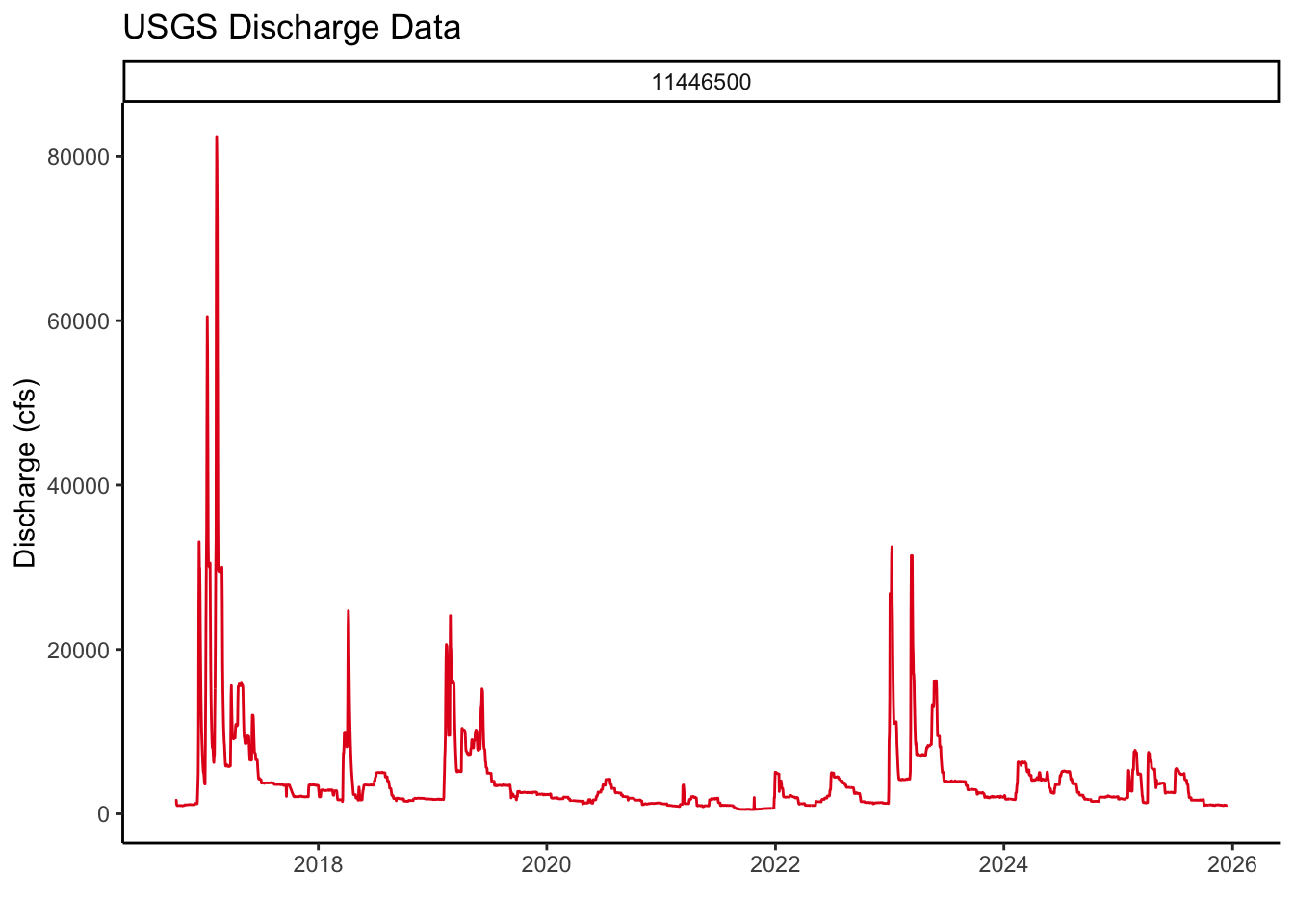
# Plot temp
(gg_temp <- ggplot() +
    geom_path(data = usgs_wTemp,
              aes(x = Date, y = Wtemp, col = site_no),
              size = .5) +
    facet_wrap(~site_no) +
    theme_bw() +
    labs(title="USGS Water Temperature Data",
         x="", y="Water Temperature (C)") +
    scale_color_viridis_d() +
    theme(legend.position = "none"))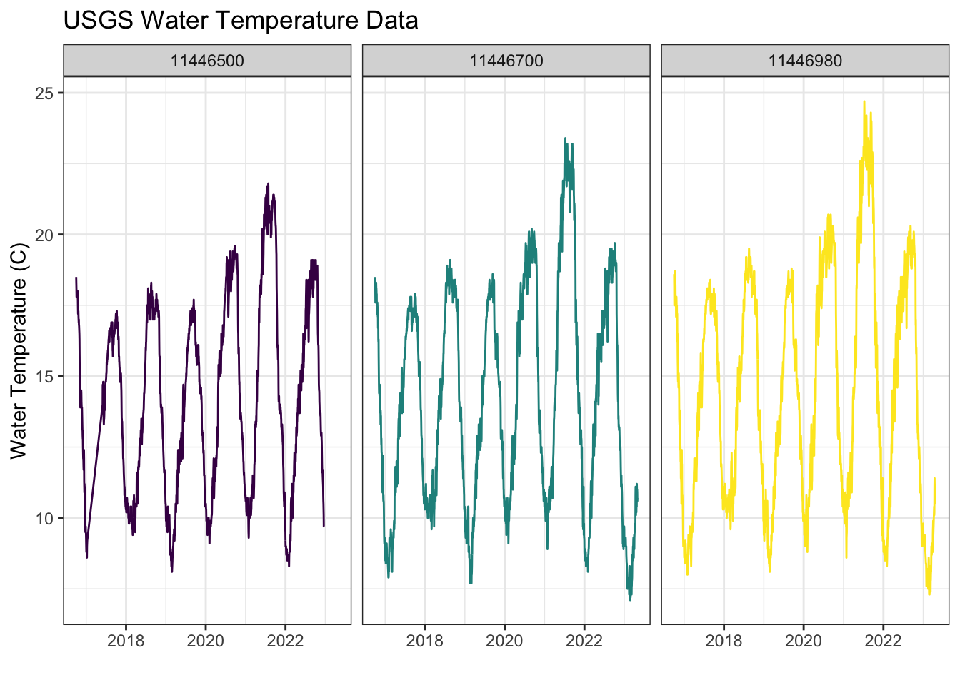
Challenge
In the plots above, we see the gaps in data are connected when using a line plot. Ideally, we would prefer to visualize these data with gaps (no line) where there is no data. To do this, we can leverage handy functions from the tidyr package: complete() and fill().
Click for Answers!
# load the package
library(tidyr)

# fill all unique combinations of Date in our data
usgs_wTemp2 <- usgs_wTemp %>%
  group_by(site_no) %>% # group by our gages first
  complete(Date = seq.Date(min(Date), max(Date), by="day")) %>%
  # then list the cols we want to fill same value through whole dataset
  fill(site_no, agency_cd)

# now regenerate plot!
# Plot temp
(gg_temp2 <- ggplot() +
    geom_path(data = usgs_wTemp2,
              aes(x = Date, y = Wtemp, col = site_no),
              size = .5) +
    facet_wrap(~site_no) +
    theme_bw() +
    labs(title="USGS Water Temperature Data",
         x="", y="Water Temperature (C)") +
    scale_color_viridis_d() +
    theme(legend.position = "none"))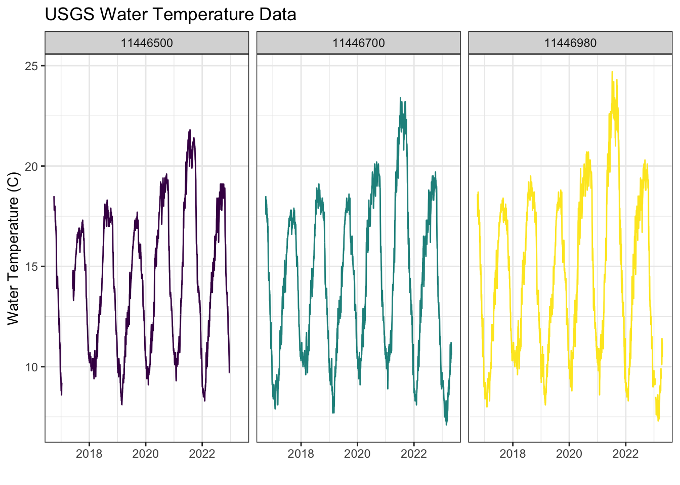
24.2 Make a Map with tmap
One final component that we haven’t covered much is how to create a publication ready-map. We can do this using the ggplot2 package in conjunction with geom_sf(), or we can use some alternate packages which are built specifically to work with spatial data and use a similar code structure to ggplot2.
The tmap and tmaptools are excellent options to create a nice map that can be used in any report or publication. First, let’s load the packages we’ll use.
library(tmap)
library(tmaptools)
Now we build our layers using a similar structure as ggplot2.
final_tmap <-

  # counties
  tm_shape(sac_co) +
  tm_polygons(border.col = "gray50", col = "gray50",
              alpha = 0.1, border.alpha = 0.9, lwd = 0.5, lty = 1) +

  # rivers
  tm_shape(us_flowlines) +
  tm_lines(col = "steelblue", lwd = 2) +

  # points: LOI stations
  tm_shape(sac_loi) +
    tm_symbols(col = "orange3", border.col = "gray20",
               shape = 21, size = 1.5, alpha = 1) +
    tm_add_legend('symbol',shape = 21, col='orange3', border.col='black', size=1,
                 labels=c(' LOI')) +
  # points usgs
  tm_shape(usgs_stations_15km) +
    tm_symbols(col = "cyan4", border.col = "gray20",
               shape = 23, size = 0.5) +
  tm_add_legend('symbol',shape = 23, col='cyan4', border.col='black', size=1,
                 labels=c(' USGS Stations')) +
  # layout
    tm_layout(
              frame = FALSE,
              legend.outside = FALSE, attr.outside = FALSE,
              inner.margins = 0.01, outer.margins = (0.01),
              legend.position = c(0.2,0.8)) +
    tm_compass(type = "4star", position = c("right","bottom")) +
    tm_scale_bar(position = c("right","bottom"))

final_tmap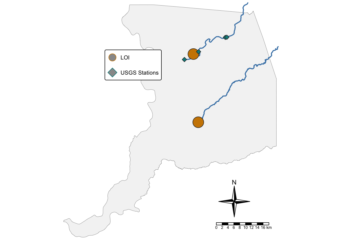
To save this map, we use a similar function as the ggsave(), but in this case, it’s tmap::tmap_save().
tmap::tmap_save(final_tmap,
                filename = "images/map_of_sites.jpg",
                height = 11, width = 8, units = "in", dpi = 300)
For more info on the NLDI: https://labs.waterdata.usgs.gov/about-nldi/index.qmd↩︎